Visualisation and dynamical systems
John Hubbard
When asked to explain what my mathematics is about, I often answer by showing pictures illustrating the behavior of the dynamical systems I study. Non-mathematicians usually respond with interest, at least polite interest but sometimes much more. They often express amazement that my pictures are in any way related to mathematics. Mathematicians are also often interested, but many (fewer as time goes on) dismiss what I do as some sort of “fad math" devoid of theorems.
Visualization can be essential even if the object is
the purest of mathematics. The pictures generated by computers using non-linear
dynamical systems may or may not be beautiful; they may or may not be art; there doesn't seem to be
a \true" answer to such questions, and each viewer must come to his or her own conclusions. But
the pictures most definitely contain information of essential interest to
mathematicians.
They help us to formulate conjectures, which in many cases would be inconceivable without the pictures. Experimentation, again using computer graphics, often can guide us to a proof, from which any computer aspect is totally absent. Finally, in the essential task of communicating our discoveries to others, the computer graphics may be absolutely essential.
Complex dynamics and visualization
I remember Lars Ahlfors, in 1982, telling me that in
his youth his adviser Ernst Lindelöf made him read the memoirs of Fatou and
Julia on the iteration of rational functions. These memoirs, he told me, struck
him at the time as “the pits of complex analysis." He said that he only
understood what they were about when seeing the pictures Mandelbrot and I were
showing. If even Ahlfors, the creator of some of the principal tools in the
field, couldn't see what the authors were getting at, what of lesser mortals?
Indeed, those memoirs were practically forgotten for 60 years, waiting for
computer graphics to reveal what Fatou and Julia had glimpsed.
The dynamics of the pendulum
I will now present a more personal example: the
movements of the forced damped pendulum, governed by the \garden-variety"
differential equation
q’’ + a q’ + b sin q = c cos(wt):
Since a robot is an assemblage of forced damped
oscillators, it is of great interest to understand the dynamical properties of
such an object. Moreover, this differential equation has been studied by
generations of students in courses in ordinary differential equations, either
as an example in perturbation theory (develop the solutions in power series
with respect to b, since the equation is linear when b = 0) or an example to
test various numerical methods. Apparently, none of these studies led to any
precise understanding of the behavior of solutions to the equation.
A bit of computer investigation for the values a = .1;
b = c = w = 1 leads to the observation that these exists
an attracting oscillation of the system of period T = 2p,
corresponding to the downward equilibrium of the unforced pendulum. But the
pendulum can get from an initial state to the attracting oscillation in many
ways, and one essential measurement of the difference between two such
evolutions is how many times the pendulum \goes over the top" before
settling down. Certainly if two evolutions correspond to different numbers of
such passages, they must be quite uncorrelated. If we color the plane of
initial states (positions and velocities) according to how many times the
pendulum goes over the top before settling down, we obtain the following
picture.

FIGURE 1. The plane of intial states colored according to the number of times the
pendulum goes over the top before settling down.
Contemplating this picture led to the conjecture that
the basins form Lakes of Wada : every point in the boundary of one is in the
boundary of all the others. When originally discovered by Brouwer and Yoneyama
[4], this sort of behavior was seen as pathological; I am sure neither thought
that such things would show up in mathematical problems of an applied nature.
Drawing the stable and unstable manifolds of the unstable periodic solution corresponding to the upper equilibrium of the pendulum leads to another conjecture: by choosing the initial condition correctly, the pendulum can be induced to go through any sequence of gyrations one wants, for instance turning once counterclockwise, then three times clockwise, then spending time almost vertical, then turning 5 billion times lockwise, and then once counterclockwise, etc.
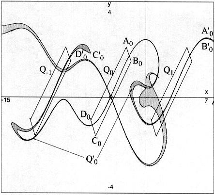
FIGURE 2. A quadrilateral in the plane of initial conditions,
with its forward and backward images going through itself three times, forming
a Smale Horseshoe. The quadrilateral is “fitted" to the unstable manifold
of an unstable equilibrium.
In both cases, with the help of the computer, the conjectures
can be proved, using techniques due to Yorke, Kennedy and Nusse [2] for the
first, and to Smale [3] for the second. The details are given in [1].
Some conclusions
This story has implications, for mathematics, for
science and engineering, and for education.
In mathematics, the use of visualization leads to
interesting conjectures, which would never have been contemplated without such
technology. The entire field of complex dynamics is filled with similar
examples: I am convinced that without computer graphics, the field would simply
not exist, and I know that in the parts I have participated in, the motivation
provided by computer graphics was essential, even if computers are never
mentioned in the proofs.
Further, as Fatou and Julia discovered, even if you can prove theorems, you often can't communicate why they are interesting without the illustrations provided by computers.
The implications for science are probably more
important yet. It is clear, from looking at the pictures and from the proofs, that the motion
of a pendulum is unstable and chaotic: the challenge is to harness this
instability to make robots more efficient. One can imagine two scenarios: a
robot moving awkwardly, frequently stopping to reset its position to within
prescribed tolerances before going on to the next task, like a beginning skier
who stops between turns to regain his balance. But exploiting the
instabilities should lead to the robot moving fluidly, expending far less
energy, like an experienced skier floating down the slope, constantly out of
balance but with effortless ease.
At the moment, robots move according to the first
scenario; they would be immensely more effective if we could move them to the
second.
Where
teaching of mathematics is concerned, I have found that computers can be
immensely successful in bringing topics to life, and any teacher of math can
attest to how essential this is: the mathematical objects students are expected
to study often, in fact usually, have no reality in the student's minds, which
prevents them from thinking about them effectively. Computers also allow the
use of far more interesting examples, much closer to real problems. The
pendulum example has been used in several undergraduate classes; this would
have been inconceivable without the computer.
Bibliography
[1] J. H. Hubbard, The Forced Damped Pendulum:
Chaos, Complication and Control, American Mathematical Monthly, 106, 8,
(1999), pp. 741-758.
[2] J. Kennedy and J. Yorke, Basins of Wada, Physica
D 51 (1991), 213-255.
[3] S. Smale, Diffeomorphisms with many periodic points, Differential and combinatorial topology, edited by S. S. Cairns, Princeton U. Press (1965) 63-80.
[4] K. Yoneyama, Theory of continuous set of points, Tohoku
Math. J., 11-12 (1917), 43.