Hyperseeing, Knots, and Minimal Surfaces
Nathaniel
A. Friedman
Department
of Mathematics
University at Albany-SUNY
Albany,
NY, 12222, USA
Abstract
We wish to highlight the fact that seeing is of basic importance in mathematics just as in art. We will introduce hyperseeing which is a more complete all-around seeing from multiple viewpoints. Hyperseeing is then applied to study knot forms and their corresponding minimal surfaces.
1. Hyperseeing
One can say that the operative word that unifies art and mathematics is SEEING. More precisely, art and mathematics are both about SEEING RELATIONSHIPS. One can see certain mathematical forms as art forms and creativity is about seeing from a new viewpoint. Thus it is all about seeing. As the Basque sculptor Eduardo Chillida states "to look is one thing, to see is another thing", "to look is to try to see", "to see is very difficult, normally" [1]. I would like to add that from my own experience as a research mathematician and sculptor, it can take a lot of looking before one finally sees what has been there all the time. Seeing better is a lifetime endeavor. An excellent related article is See-Duction by Howard Levine [2].
We will now discuss a more complete way of seeing a three-dimensional object that is called hyperseeing. First we note that to see a two-dimensional painting on a wall, we step back from the wall in a third dimension. We then see the shape of the painting ( generally rectangular ) as well as every point in the painting. Thus we see the painting completely from one viewpoint. Now theoretically, in order to see a three-dimensional object completely from one viewpoint, we would need to step back in a fourth spatial dimension. From one viewpoint, we could then (theoretically) see every point on the object, as well as every point within the object. This type of all-around seeing, as well as a type of x-ray seeing, was known to the Cubist painters such as Braque, Duchamp, and Picasso, as discussed in [3]. In particular, Cubists were led to showing multiple views of an object in the same painting. In mathematics four-dimensional space is referred to as hyperspace and I refer to seeing in hyperspace as hyperseeing ([4]-[7]). Thus in hyperspace one could hypersee a three-dimensional object completely from one viewpoint. The Cubists were approximating hyperseeing in their paintings with multiple views. In general, we can regard hyperseeing in our own three-dimensional world as a more complete all-around seeing from multiple viewpoints. We will apply hyperseeing to study knots and their soapfilm minimal surfaces.
2. Knots
Knots are usually presented by two-dimensional knot
diagrams that indicate where the knot crosses itself. Three diagrams of a trefoil knot are shown in Figure 1.
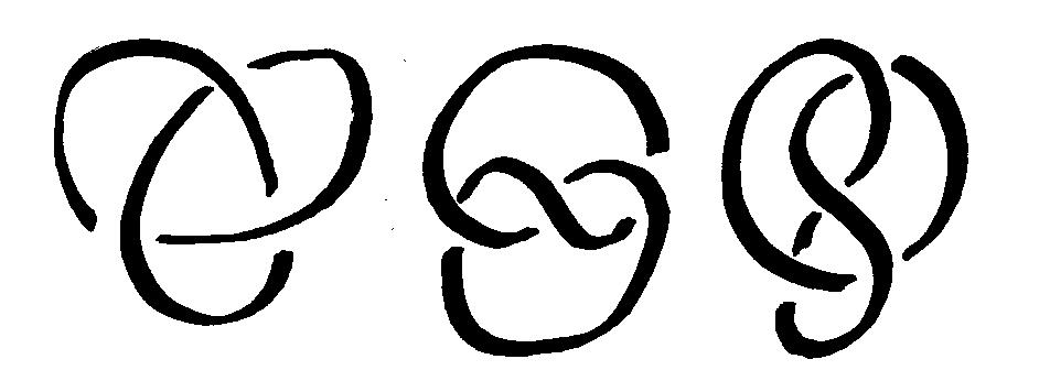
Figure 1. Trefoil Diagrams
Knots are usually presented as two-dimensional knot diagrams. However, a knot is actually a three-dimensional object and a knot really comes alive in a three-dimensional model of the knot which can be constructed from wire, folded aluminium foil, folded aluminium foil with a wire insert, copper tubing , or other material. Models of knots are ideal mathematical forms that can generate ideas for sculptures. Examples of models of knots made from folded aluminium foil are shown in Figure 2. A knot made from copper tubing is shown in Figure 3.

Figure 2. Aluminum Foil Knots

Figure 3. Copper Tubing Knot
Models of
knots are perfect mathematical forms for generating ideas for sculptures. They
are completely three-dimensional with no preferred top, bottom, front, or back.
Furthermore, a knot can look completely different when viewed from different
directions. John Robinson has made beautiful bronze sculptures based on knot
forms ( see Sculpture in the Directory at www.isama.org
).
As mentioned above, we can regard hyperseeing in our three-dimensional world as a more complete all-around seeing from multiple viewpoints. Since knots can look so different from different viewpoints, knots are excellent examples of interesting forms on which to practice hyperseeing. Knots are also open forms that one can actually see through. This is another reason that knots are ideal forms for hyperseeing.
For example, if one makes a wire model of a trefoil
knot with front view as in Figure 1(a), then the top view will appear similar
to Figure 1(b). A right side view of the model with a little tip forward will
appear similar to Figure 1(c). In general, a model of a knot yields an infinite
number of diagrams of the knot depending on your viewpoint of the knot.
There are
several interesting mathematical
exercises related to hyperseeing a model of a knot. For example, every knot
admits a quadra secant. This is a viewpoint where one sees a diagram containing
a point where four arcs of the knot coincide.
Normally a crossing is where two arcs coincide. Colin Adams has
introduced an exercise where the model is placed inside a plastic sphere and
one maps the regions on the sphere corresponding to how many crossings one sees
viewing the knot from a point in the region. For a trefoil knot there will be regions
corresponding to at least three crossings. Adams has conjectured that a model
of a trefoil knot always admits a viewpoint with a diagram having six
crossings. In particular, this will imply that a trefoil model will admit viewpoints with diagrams having n
crossings, n = 3,4,5, and 6. A projection of a knot is a diagram of a knot with
the crossings not indicated as under/ over. Thus a projection corresponds to
replacing crossings by just intersections of two arcs.. That is, a projection
is just a "shadow" of a knot. The crossing number c(K) of a knot K is
the least number of crossings that occur in a diagram of K. For example, if K
is a trefoil knot, then c(K) = 3. If K
is a loop, then c(K) = 0. Knots are
listed in knot tables according to their crossing numbers.
When we hypersee a knot model from different
viewpoints, we obtain a variety of diagrams. Given a diagram, we can consider
the corresponding projection. Given a projection with n crossings, one can
assign under/over at each crossing. This will yield a variety of knots with
crossing numbers between 0 and n. One can always assign crossings so that the
one obtains a loop with crossing number 0. In the reduced case ([8], page 68),
one can also assign the crossings to obtain an alternating knot with crossing
number n. Therefore given a knot model,
one can choose a viewpoint and obtain a diagram with n crossings. By changing
the crossings , one obtains knot diagrams with a variety of crossing numbers
between 0 and n. Thus one viewpoint yields a variety of knots. In particular, a
trefoil model can have viewpoints
yielding diagrams of knots with crossing number between 0 and 6.
An interesting property that results from the open
structure of a knot concerns looking at a model of a knot from opposite directions. Suppose we regard one viewpoint as
the front viewpoint. The viewpoint directly opposite will be the rear
view. In general, the rear view of an
object cannot be determined at all from the front view. However, for a knot,
the rear view will be the reflection of the front view with the crossings
reversed. For example, if one considers the views in Figure 1 as front views,
then the corresponding rear views can be obtained by holding the turned page to
the light and reversing the crossings.
Another property of knots is that one sees all points on a knot in any one view except for a finite number of crossing points. This implies that front and top views determine the side views . To see why this is true, let us fix one point P on the knot in an x,y,z coordinate system. A view along the x-axis determines the y and z coordinates of P. A view along the y-axis determines the x and z coordinates of P. Thus two orthogonal views determine the x,y,z coordinates of P in space. Applying this to points P on a knot, it folows that two orthogonal views of a knot will determine the position of the knot in space. In particular, the front and top views determine the side view. This is an interesting exercise in hyperseeing the knot. A suggested first exercise is to consider a straight line in space with endpoints P = (a,b,c) and Q= (d,e,f). A view along the x-axis shows P at (b,c) and Q at (e,f) . A view along the z-axis shows P at (a,b) and Q at (d,e). The view along the y-axis is therefore determined with P at (a,c) and Q at (d,f). One can now connect (a,c) and (d,f) by a straight line to obtain the side view of the line. An example of a triangle in space is shown in Figure 4, where the side view is from the left.
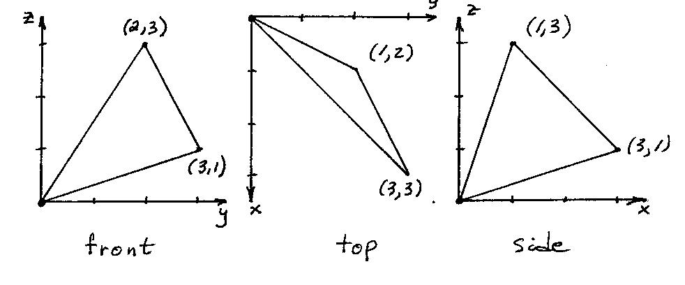
Figure 4. Front, Top, and Side Views
The next
exercise is to consider a knot formed
by straight line segments. One can then
obtain the side view from front and top
views using coordinates of the endpoints of the lines. No line can be parallel
to an x,y, or z axis.
3. Kenneth
Snelson Sculptures
Kenneth Snelson sculptures consist of line elements
suspended in space. For example, Free Ride
Home is shown in Figure 5. The discussion above
implies that a front and top view of a
Snelson sculpture would determine the side view.

Figure 5. Free Ride Home, Kenneth Snelson, 1974,
Stormking Art Center, Mountainville , New York
4. Soapfilm Minimal Surfaces of Knots
If one dips a wire model of a knot in a solution of
liquid soap and water, one obtains a soapfilm minimal surface with the knot as
the single edge of the surface. For example, the edge of a half-twist Mobius band is a simple loop as
shown in Figure 6(a). If a wire is bent in this shape and dipped in a soap
solution, one obtains a minimal surface with a central disk. If this disk is
puntcured, then one obtains the Mobius band minimal surface in Figure 6(b).

The
corresponding soapfilm minimal surfaces
for the trefoil knots in Figure 1
are shown in Figure 7. In (a) we have a triple twist Mobius band with
one side. In (b) we have a two-sided minimal surface. In (c) we have a one-sided minimal surface. 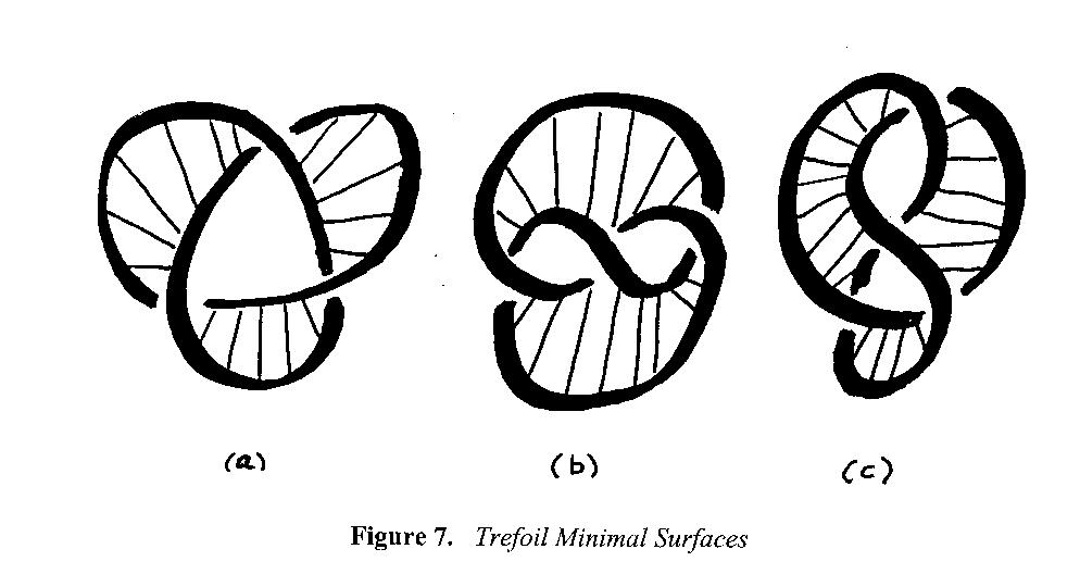
The exercise students of all ages really enjoy is
dipping wire models of knots in order to obtain the corresponding soapfilm
minimal surfaces. In order that students can learn to anticipate the shape of
the surface, it is helpful to use masking tape in order to approximate the
surface. An example is shown in Figure
8 for a trefoil knot.
.
5. Framed Knots
In Figure 7(a) we have a minimal surface that could be described as a form consisting of three leaves with a central space. We will now modify the knot so that the leaves become space and the center is form. The modified knot is shown in Figure 9(a) and the corresponding minimal surface is shown in (b). We refer to the knot in (a) as a framed knot. The original idea is to form a link obtained by placing the knot inside a circle. This was first shown to me by the sculptor Charles Perry. Later I saw this link in several books on knots. This led me to the idea of a framed knot. From a mathematical point of view the framed knot is not much different from the original knot since it is easy to see that one can deform the framed knot by lowering the added "frame" to obtain the original knot. However, from a sculptural viewpoint, the framed knot is interesting since it has a minimal surface that reverses form and space in the minimal surface of the original knot. One can also suspend a wire knot in a wire circle using an extra piece of wire to suspend the knot. This is the form that Charles Perry introduced in order to obtain a sculpture where form and space are switched . Perry forms the surface using flexible metal screen and then applies automobile body putty on the screen. A mold is made and then the minimal surface is cast in bronze. The idea of forming a sculpture from the minimal surface of a framed knot or a knot in a circle is a very recent development.

Figure 9. Framed Trefoil
6. Multiple Mobius Bands
In Figure 6(b) we have a minimal surface for a loop that consists of one Mobius band . It will now be shown that there is a configuration of a trefoil knot that has a minimal surface consisting of two Mobius bands that share part of their edges as in Figure 10(a) and also alternately cross over each other as in Figure 10(b). The knot is shown in Figure 11(a). In Figure 11(b) Mobius band 1 is shown and in Figure 11(c) Mobius band 2 is shown. The intersection lines on the cross overs are indicated by dotted lines.

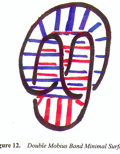
If Figures 11 (b) and (c) are combined, then we obtain the complete minimal surface shown in Figure 12. The two bands share parts of their edges and alternately cross over each other. Band 1 crosses over band 2 at the top and band 2 crosses over band 1 at the bottom. It is interesting to see each soapfilm Mobius band twist as it crosses over the other Mobius band. The bands share edges until they twist.
twist.
The knot in
Figures 10 and 11 is the representation of a trefoil knot as the 2-3 torus knot.
In general, given p and q mutually prime, the p-q torus knot wraps meridionally
around the torus p times and wraps longitudinally around the torus q times. The
p-q torus knot is equivalent to the q-p
torus knot. That is, one is deformable into the other ( see [8], page 111 ).
Thus from a mathematical viewpoint, the p-q and q-p torus knots are the same knot.However, from a sculptural
viewpoint, they look quite different and they have configurations with very
different minimal surfaces. In particular, the 3-2 torus knot is shown in Figure 1(a) and it has a minimal surface
as in Figure 7(a), which is a triple twist Mobius band. In Figure 11 we have the 2-3 torus knot with
a configuration having a minimal surface consisting of two single twist Mobius
bands. In general, the n-(n+1) torus knot has a configuration with a minimal
surface consisting of n single twist Mobius bands that partly share edges and
alternately cross over each other.
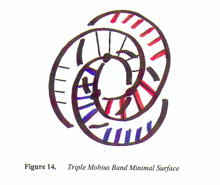
For example, the 3-4 torus knot has a minimal surface consisting of three single twist Mobius bands. Suppose we color these three bands red, white, and blue. Part of the surface will have the red band and white band sharing an edge with the red band to the left of the white band. The blue band will be crossing over the red and white bands. The blue band will then twist and share an edge with the white band, where the white band is now to the left of the blue band. The red band will now twist and cross over the white and blue bands. This structure goes around a central space so that each band twists once to cross the other two bands. In order to picture this, we will first draw the 3-4 torus knot as in Figure 13. We begin with three points as in (a). We then draw arcs as in (b). The knot is completed as in (c). The corresponding minimal surface is shown in Figure 14.

In general, the behavior of minimal surfaces for
configurations of (n+1)-n torus knots
may consist of one or more bands with one or more half twists. In Figure 7(a) for the 3-2 torus knot we
have one band with three half twists. The 4-3 torus knot has a minimal surface
consisting of two bands that partly share edges and cross over each other
twice, hence each band has two half twists. The 5-4 torus knot has a minimal surface that consists of one band that
crosses itself five times as it wraps around four times. Part of the surface
will appear as described above for the 3-4 torus knot except there is only one
band alternately crossing over itself as it wraps around.
REFERENCES
[1] E.
Chillida, Basque Sculptor, Video, Home Vision, 24, (1985).
[2] H.
Levine, See-Duction, Humanistic Mathematics Network Journal #15, (1997).
[3] L.D. Henderson, The Fourth Dimension and
Non-Euclidean Geometry in Modern Art, Princeton University Press, (1983).
[4] N.A. Friedman, Hyperspace, Hyperseeing,
Hypersculptures, Conference Proceedings, Mathematics and Design 98, Javier
Barrallo, Editor, San Sebastian, Spain.
[5] N.A. Friedman, Hyperseeing,
Hypersculptures, and Space Curves, Conference Proceedings, 1998 Bridges: Mathematical Connections in Art, Music, and
science, Reza Sarhangi, Editor, Winfield, Kansas, USA.
[6] N.A. Friedman, Hyperspace, Hyperseeing,
Hypersculptures (with figures), Hyperspace, volume 7, 1998, Japan Institute of
Hyperspace Science, Kyoto, Japan.
[7] N.A. Friedman, Geometric Sculptures for
K-12: Geos, Hyperseeing,
Hypersculptures, Conference Proceedings, 1999 Bridges: Mathematical Connections in Art, Music, and
Science, Reza Sarhangi, Editor, Winfield, Kansas, USA.
[8] C.
Adams, The Knot Book , W.H.Freeman, New York, (1994)